Excel Macros How to Use Relative References

“Relative references” sounds complicated but it’s really not. If you’re new to Macros then check out the beginner tutorial here.

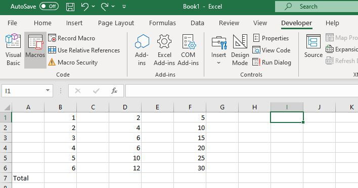
The best way to explain Relative references is to create a sample data set like the one below in Excel. Simply click and drag your mouse over the spreadsheet below and copy and paste it into Excel.

	1		2		5
	2		4		10
	3		6		15
	4		8		20
	5		10		25
	6		12		30
Total

It should look something like the table below:

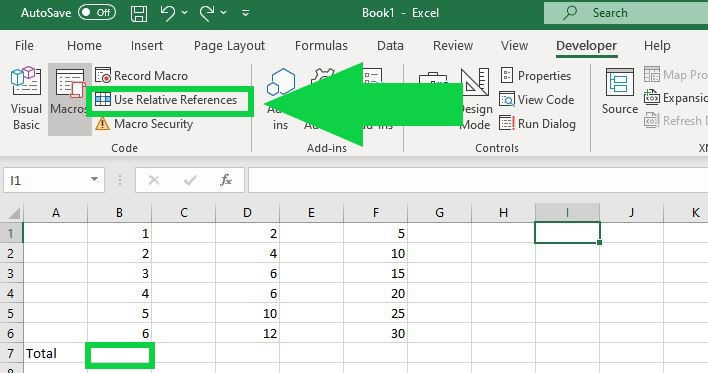
Next select cell B7 and click on “Use Relative References.”

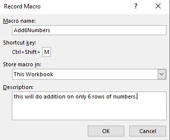
Then click on, “Record Macro.” And enter in this information:

Hit “OK.” You are now in recording mode.

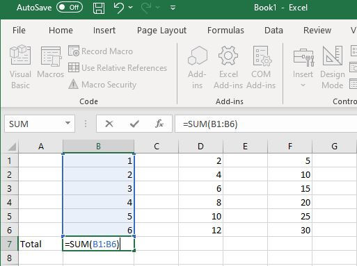
Next, type in cell B7 the following formula and hit the Enter key.

=SUM(B1:B6)

Go to “Stop Recording Macro” and that’s all you need.

Now that you have recorded your macro, you can select cell D7 and run your macro by using the shortcut CTRL + SHIFT + M.

Do this and it will add up the rows. Or you can run it manually by hitting “Macros” and running the macro from the list.

So what is Releative reference? Well if you made this macro without relative reference, it would just keep summing up the B column again and again. Which would be no use, since we want to add up the D column and the F column.

Relative reference allows you to use your macro anywhere vs in a fixed cell location.

The macro we created is useful if you have 6 rows of numbers you want to add up.